• 개발 환경(OS): Windows 10 Education, 64비트 운영 체제, x64 기반 프로세서

Library version check

import sys
import sktime
import tqdm as tq
import xgboost as xgb
import matplotlib
import seaborn as sns
import sklearn as skl
import pandas as pd
import numpy as np
print("-------------------------- Python & library version --------------------------")
print("Python version: {}".format(sys.version))
print("pandas version: {}".format(pd.__version__))
print("numpy version: {}".format(np.__version__))
print("matplotlib version: {}".format(matplotlib.__version__))
print("tqdm version: {}".format(tq.__version__))
print("sktime version: {}".format(sktime.__version__))
print("xgboost version: {}".format(xgb.__version__))
print("seaborn version: {}".format(sns.__version__))
print("scikit-learn version: {}".format(skl.__version__))
print("------------------------------------------------------------------------------")
-------------------------- Python & library version --------------------------
Python version: 3.8.8 (default, Apr 13 2021, 15:08:03) [MSC v.1916 64 bit (AMD64)]
pandas version: 1.2.4
numpy version: 1.19.2
matplotlib version: 3.3.4
tqdm version: 4.59.0
sktime version: 0.6.1
xgboost version: 1.2.1
seaborn version: 0.11.1
scikit-learn version: 0.24.2
------------------------------------------------------------------------------

0. load the libararies

import matplotlib.pyplot as plt
from tqdm import tqdm
from sktime.forecasting.model_selection import temporal_train_test_split
from sktime.utils.plotting import plot_series
from xgboost import XGBRegressor

pd.set_option('display.max_columns', 30)

1. preprocessing the data

- time series를 일반 regression 문제로 변환하기 위해 시간 관련 변수 추가(월 / 주 / 요일)
- 전력소비량의 건물별 요일별 시간대별 평균 / 건물별 시간대별 평균 / 건물별 시간대별 표준편차 변수 추가
건물별 요일별 시간대별 표준편차 / 건물별 평균 등 여러 통계량 생성 후 몇개 건물에 테스트, 최종적으로 성능 향상에 도움이 된 위 3개 변수만 추가
- 공휴일 변수 추가
- 시간(hour)는 cyclical encoding하여 변수 추가(sin time & cos time) 후 삭제
- CDH(Cooling Degree Hour) & THI(불쾌지수) 변수 추가
- 건물별 모델 생성 시 무의미한 태양광 발전 시설 / 냉방시설 변수 삭제
train = pd.read_csv('./data/train.csv', encoding = 'cp949')

## 변수들을 영문명으로 변경
cols = ['num', 'date_time', 'power', 'temp', 'wind','hum' ,'prec', 'sun', 'non_elec', 'solar']
train.columns = cols

# 시간 관련 변수들 생성
date = pd.to_datetime(train.date_time)
train['hour'] = date.dt.hour
train['day'] = date.dt.weekday
train['month'] = date.dt.month
train['week'] = date.dt.weekofyear

#######################################
## 건물별, 요일별, 시간별 발전량 평균 넣어주기
#######################################
power_mean = pd.pivot_table(train, values = 'power', index = ['num', 'hour', 'day'], aggfunc = np.mean).reset_index()
tqdm.pandas()
train['day_hour_mean'] = train.progress_apply(lambda x : power_mean.loc[(power_mean.num == x['num']) & (power_mean.hour == x['hour']) & (power_mean.day == x['day']) ,'power'].values[0], axis = 1)

#######################################
## 건물별 시간별 발전량 평균 넣어주기
#######################################
power_hour_mean = pd.pivot_table(train, values = 'power', index = ['num', 'hour'], aggfunc = np.mean).reset_index()
tqdm.pandas()
train['hour_mean'] = train.progress_apply(lambda x : power_hour_mean.loc[(power_hour_mean.num == x['num']) & (power_hour_mean.hour == x['hour']) ,'power'].values[0], axis = 1)

#######################################
## 건물별 시간별 발전량 표준편차 넣어주기
#######################################
power_hour_std = pd.pivot_table(train, values = 'power', index = ['num', 'hour'], aggfunc = np.std).reset_index()
tqdm.pandas()
train['hour_std'] = train.progress_apply(lambda x : power_hour_std.loc[(power_hour_std.num == x['num']) & (power_hour_std.hour == x['hour']) ,'power'].values[0], axis = 1)

### 공휴일 변수 추가
train['holiday'] = train.apply(lambda x : 0 if x['day']<5 else 1, axis = 1)
train.loc[('2020-08-17'<=train.date_time)&(train.date_time<'2020-08-18'), 'holiday'] = 1

## https://dacon.io/competitions/official/235680/codeshare/2366?page=1&dtype=recent
train['sin_time'] = np.sin(2*np.pi*train.hour/24)
train['cos_time'] = np.cos(2*np.pi*train.hour/24)

## https://dacon.io/competitions/official/235736/codeshare/2743?page=1&dtype=recent
train['THI'] = 9/5*train['temp'] - 0.55*(1-train['hum']/100)*(9/5*train['hum']-26)+32

def CDH(xs):
    ys = []
    for i in range(len(xs)):
        if i < 11:
            ys.append(np.sum(xs[:(i+1)]-26))
        else:
            ys.append(np.sum(xs[(i-11):(i+1)]-26))
    return np.array(ys)

cdhs = np.array([])
for num in range(1,61,1):
    temp = train[train['num'] == num]
    cdh = CDH(temp['temp'].values)
    cdhs = np.concatenate([cdhs, cdh])
train['CDH'] = cdhs

train.drop(['non_elec','solar','hour'], axis = 1, inplace = True)
train.head()
<ipython-input-3-b79acc44fcb3>:12: FutureWarning: Series.dt.weekofyear and Series.dt.week have been deprecated.  Please use Series.dt.isocalendar().week instead.
  train['week'] = date.dt.weekofyear
100%|████████████████████████████████████████████████████████████████████████| 122400/122400 [01:09<00:00, 1750.29it/s]
100%|████████████████████████████████████████████████████████████████████████| 122400/122400 [00:43<00:00, 2809.77it/s]
100%|████████████████████████████████████████████████████████████████████████| 122400/122400 [00:43<00:00, 2811.58it/s]
num date_time power temp wind hum prec sun day month week day_hour_mean hour_mean hour_std holiday sin_time cos_time THI CDH
0 1 2020-06-01 00 8179.056 17.6 2.5 92.0 0.8 0.0 0 6 23 8528.627077 8540.373176 118.793252 0 0.000000 1.000000 57.5376 -8.4
1 1 2020-06-01 01 8135.640 17.7 2.9 91.0 0.3 0.0 0 6 23 8513.723077 8517.174776 137.989738 0 0.258819 0.965926 57.0389 -16.7
2 1 2020-06-01 02 8107.128 17.5 3.2 91.0 0.0 0.0 0 6 23 8496.625846 8509.055718 122.381197 0 0.500000 0.866025 56.6789 -25.2
3 1 2020-06-01 03 8048.808 17.1 3.2 91.0 0.0 0.0 0 6 23 8480.076923 8493.313129 122.054777 0 0.707107 0.707107 55.9589 -34.1
4 1 2020-06-01 04 8043.624 17.0 3.3 92.0 0.0 0.0 0 6 23 8472.051692 8479.522165 124.472447 0 0.866025 0.500000 56.4576 -43.1
## save the preprocessed data
train.to_csv('./data/train_preprocessed.csv')

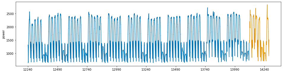
sktime library으로 마지막 일주일을 validation set으로 설정

## 7번 건물의 발전량
y = train.loc[train.num == 7, 'power']
x = train.loc[train.num == 7, ].iloc[:, 3:]

y_train, y_valid, x_train, x_valid = temporal_train_test_split(y = y, X = x, test_size = 168) # 24시간*7일 = 168

print('train data shape\nx:{}, y:{}'.format(x_train.shape, y_train.shape))

plot_series(y_train, y_valid, markers=[',' , ','])
plt.show()
train data shape
x:(1872, 16), y:(1872,)

2. Model : XGBoost

모델은 시계열 데이터에 좋은 성능을 보이는 XGBoost를 선정했습니다.

# Define SMAPE loss function
def SMAPE(true, pred):
    return np.mean((np.abs(true-pred))/(np.abs(true) + np.abs(pred))) * 100

아래와 같이 평가 Metric인 SMAPE는 실제값보다 작게 추정할 때 더 좋지 않습니다.

이는 전력사용량을 높게 예측하는 것보다 작게 예측할 때 실제로 더 큰 문제가 될 수 있음을 반영한 것으로 보입니다.

print("실제값이 100일 때 50으로 underestimate할 때의 SMAPE : {}".format(SMAPE(100, 50)))
print("실제값이 100일 때 150으로 overestimate할 때의 SMAPE : {}".format(SMAPE(100, 150)))
실제값이 100일 때 50으로 underestimate할 때의 SMAPE : 33.33333333333333
실제값이 100일 때 150으로 overestimate할 때의 SMAPE : 20.0

그러나 일반 mse를 objective function으로 훈련할 때 과소추정하는 건물들이 있음을 확인했습니다.

이때문에 SMAPE 점수가 높아진다고 판단, 이를 해결하기 위해 아래와 같이 objective function을 새로 정의했습니다.

새 목적함수는 residual이 0보다 클 때, 즉 실제값보다 낮게 추정할 때 alpha만큼의 가중치를 곱해 반영합니다.

XGBoost는 custom objective function으로 훈련하기 위해선 아래와 같이

gradient(1차 미분함수) / hessian(2차 미분함수)를 정의해 두 값을 return해주어야 합니다.

#### alpha를 argument로 받는 함수로 실제 objective function을 wrapping하여 alpha값을 쉽게 조정할 수 있도록 작성했습니다.
# custom objective function for forcing model not to underestimate
def weighted_mse(alpha = 1):
    def weighted_mse_fixed(label, pred):
        residual = (label - pred).astype("float")
        grad = np.where(residual>0, -2*alpha*residual, -2*residual)
        hess = np.where(residual>0, 2*alpha, 2.0)
        return grad, hess
    return weighted_mse_fixed
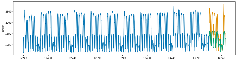
기본 mse를 objective function으로 사용할 때 : SAMPE 12.7705
xgb_params = pd.read_csv('./parameters/hyperparameter_xgb.csv')

xgb_reg = XGBRegressor(n_estimators = 10000, eta = xgb_params.iloc[47,1], min_child_weight = xgb_params.iloc[47,2], 
                       max_depth = xgb_params.iloc[47,3], colsample_bytree = xgb_params.iloc[47,4], 
                       subsample = xgb_params.iloc[47,5], seed=0)

xgb_reg.fit(x_train, y_train, eval_set=[(x_train, y_train), (x_valid, y_valid)],
        early_stopping_rounds=300,
       verbose=False)
XGBRegressor(base_score=0.5, booster='gbtree', colsample_bylevel=1,
             colsample_bynode=1, colsample_bytree=0.8, eta=0.01, gamma=0,
             gpu_id=-1, importance_type='gain', interaction_constraints='',
             learning_rate=0.00999999978, max_delta_step=0, max_depth=5,
             min_child_weight=6, missing=nan, monotone_constraints='()',
             n_estimators=10000, n_jobs=0, num_parallel_tree=1, random_state=0,
             reg_alpha=0, reg_lambda=1, scale_pos_weight=1, seed=0,
             subsample=0.9, tree_method='exact', validate_parameters=1,
             verbosity=None)
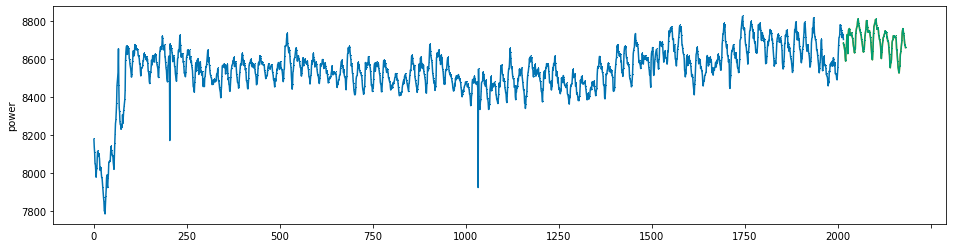
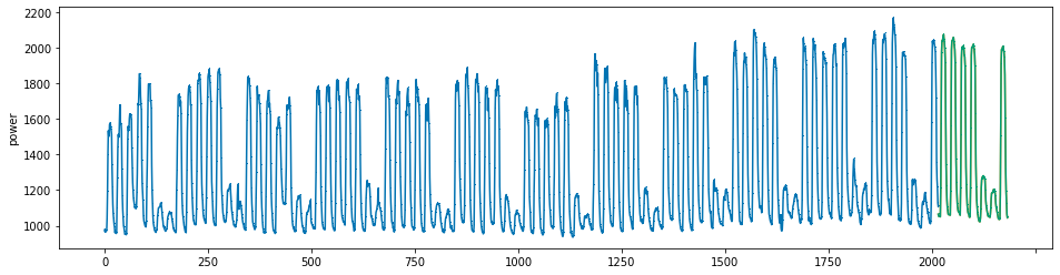
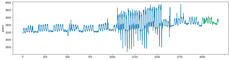
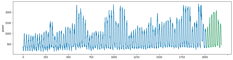
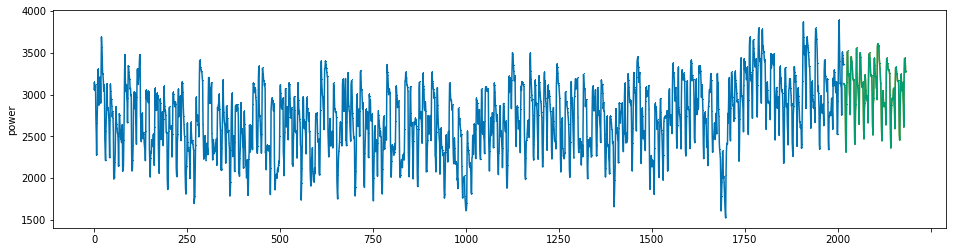
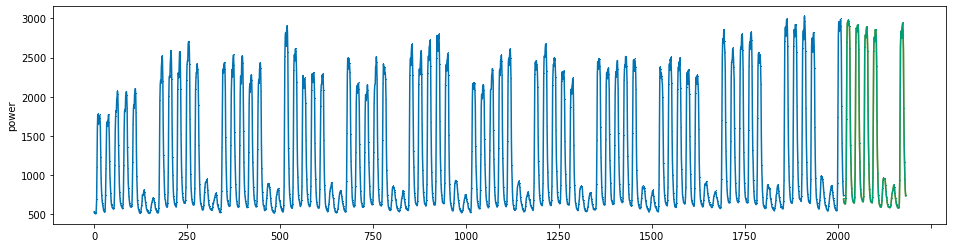
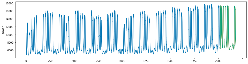
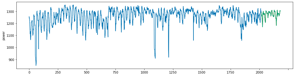
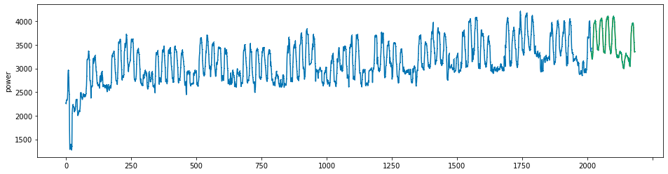
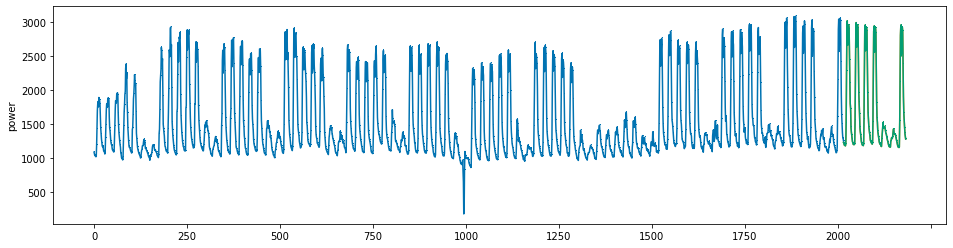
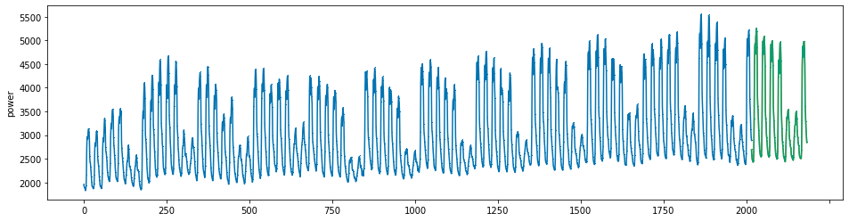
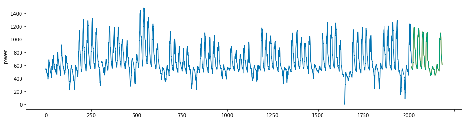
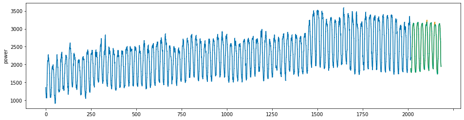
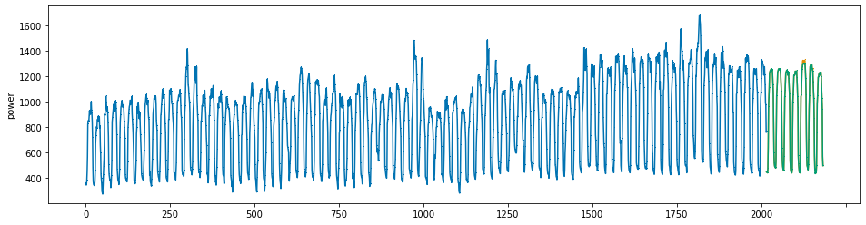
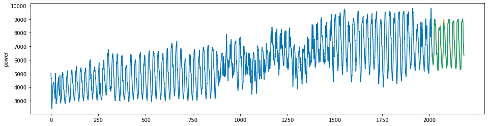
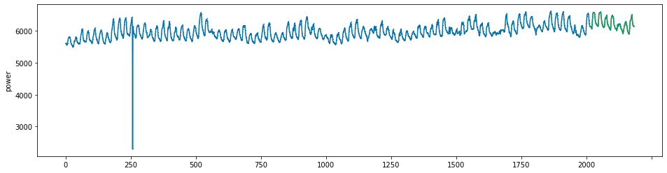
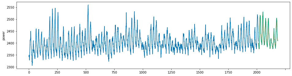
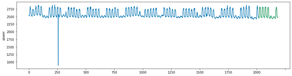
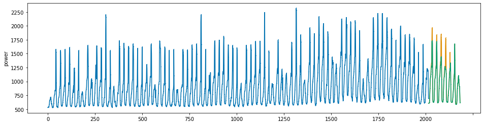
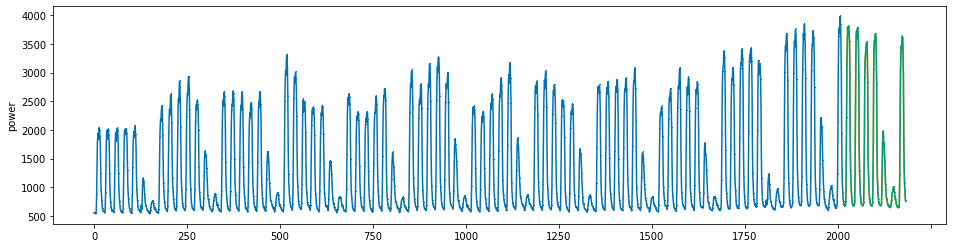
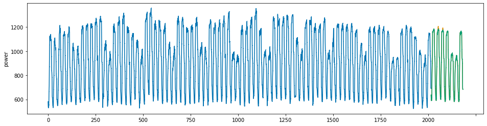
## 주황색이 실제 전력소비량, 초록색이 예측값입니다.
pred = xgb_reg.predict(x_valid)
pred = pd.Series(pred)
pred.index = np.arange(y_valid.index[0], y_valid.index[-1]+1)
plot_series(y_train, y_valid, pd.Series(pred), markers=[',' , ',', ','])

print('best iterations: {}'.format(xgb_reg.best_iteration))
print('SMAPE : {}'.format(SMAPE(y_valid, pred)))
best iterations: 496
SMAPE : 12.770522968347997
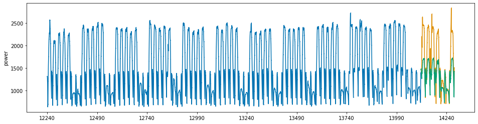
with weighted mse(alpha = 100) : SMAPE 9.9390
xgb_reg = XGBRegressor(n_estimators = 10000, eta = xgb_params.iloc[47,1], min_child_weight = xgb_params.iloc[47,2], 
                       max_depth = xgb_params.iloc[47,3], colsample_bytree = xgb_params.iloc[47,4], 
                       subsample = xgb_params.iloc[47,5], seed=0)

xgb_reg.set_params(**{'objective':weighted_mse(100)})

xgb_reg.fit(x_train, y_train, eval_set=[(x_train, y_train), (x_valid, y_valid)],
        early_stopping_rounds=300,
       verbose=False)
XGBRegressor(base_score=0.5, booster='gbtree', colsample_bylevel=1,
             colsample_bynode=1, colsample_bytree=0.8, eta=0.01, gamma=0,
             gpu_id=-1, importance_type='gain', interaction_constraints='',
             learning_rate=0.00999999978, max_delta_step=0, max_depth=5,
             min_child_weight=6, missing=nan, monotone_constraints='()',
             n_estimators=10000, n_jobs=0, num_parallel_tree=1,
             objective=<function weighted_mse.<locals>.weighted_mse_fixed at 0x0000027A73C84EE0>,
             random_state=0, reg_alpha=0, reg_lambda=1, scale_pos_weight=1,
             seed=0, subsample=0.9, tree_method='exact', validate_parameters=1,
             verbosity=None)
## SMAPE 값으로도, 그래프 상으로도 과소추정이 모델이 개선되었음을 확인
pred = xgb_reg.predict(x_valid)
pred = pd.Series(pred)
pred.index = np.arange(y_valid.index[0], y_valid.index[-1]+1)
plot_series(y_train, y_valid, pd.Series(pred), markers=[',' , ',', ','])

print('best iterations: {}'.format(xgb_reg.best_iteration))
print('SMAPE : {}'.format(SMAPE(y_valid, pred)))
best iterations: 723
SMAPE : 9.939030437541014

3. model tuning

다른 parameter를 고정하지 않고 전체 parameter를 튜닝하고자 하면 매우 오래걸리기 때문에

모델 내 hyperparameter들은 아래와 같이 sklearn의 gridsearchCV를 활용해 튜닝하고,

XGBoost의 early stopping 기능으로 n_estimators를 튜닝하고,

weighted_mse의 alpha값을 튜닝했습니다.

참고

gridsearch 코드는 빠른 튜닝을 위해 NIPA서버를 활용해 gpu버전으로 튜닝하여 cpu버전으로 찾은 parameter와는 값이 다릅니다.
(gpu와 cpu버전의 bootstrap 과정 등의 차이에 기인하는 것으로 생각됩니다.)
그러므로 gridsearchCV 코드는 제출하되 튜닝된 parameter를 csv로 첨부합니다.
이후 모든 과정은 첨부된 csv에 저장된 paramter를 사용하여 훈련, 예측합니다.
## gridsearchCV for best model : 대략 1시간 소요
"""
from sklearn.model_selection import PredefinedSplit, GridSearchCV
df = pd.DataFrame(columns = ['n_estimators', 'eta', 'min_child_weight','max_depth', 'colsample_bytree', 'subsample'])
preds = np.array([])

grid = {'n_estimators' : [100], 'eta' : [0.01], 'min_child_weight' : np.arange(1, 8, 1), 
        'max_depth' : np.arange(3,9,1) , 'colsample_bytree' :np.arange(0.8, 1.0, 0.1), 
        'subsample' :np.arange(0.8, 1.0, 0.1)} # fix the n_estimators & eta(learning rate)
        
for i in tqdm(np.arange(1, 61)):
    y = train.loc[train.num == i, 'power']
    x = train.loc[train.num == i, ].iloc[:, 3:]
    y_train, y_test, x_train, x_test = temporal_train_test_split(y = y, X = x, test_size = 168)
    
    
    pds = PredefinedSplit(np.append(-np.ones(len(x)-168), np.zeros(168)))
    gcv = GridSearchCV(estimator = XGBRegressor(seed = 0, gpu_id = 1, 
                                                tree_method = 'gpu_hist', predictor= 'gpu_predictor'),
                       param_grid = grid, scoring = smape, cv = pds, refit = True, verbose = True)
    
    
    gcv.fit(x_train, y_train)
    best = gcv.best_estimator_
    params = gcv.best_params_
    print(params)
    pred = best.predict(x_test)
    building = 'building'+str(i)
    print(building + '|| SMAPE : {}'.format(SMAPE(y_test, pred)))
    preds = np.append(preds, pred)
    df = pd.concat([df, pd.DataFrame(params, index = [0])], axis = 0)
    df.to_csv('./hyperparameter_xgb.csv', index = False) # save the tuned parameters
"""
"\nfrom sklearn.model_selection import PredefinedSplit, GridSearchCV\ndf = pd.DataFrame(columns = ['n_estimators', 'eta', 'min_child_weight','max_depth', 'colsample_bytree', 'subsample'])\npreds = np.array([])\n\ngrid = {'n_estimators' : [100], 'eta' : [0.01], 'min_child_weight' : np.arange(1, 8, 1), \n        'max_depth' : np.arange(3,9,1) , 'colsample_bytree' :np.arange(0.8, 1.0, 0.1), \n        'subsample' :np.arange(0.8, 1.0, 0.1)} # fix the n_estimators & eta(learning rate)\n        \nfor i in tqdm(np.arange(1, 61)):\n    y = train.loc[train.num == i, 'power']\n    x = train.loc[train.num == i, ].iloc[:, 3:]\n    y_train, y_test, x_train, x_test = temporal_train_test_split(y = y, X = x, test_size = 168)\n    \n    \n    pds = PredefinedSplit(np.append(-np.ones(len(x)-168), np.zeros(168)))\n    gcv = GridSearchCV(estimator = XGBRegressor(seed = 0, gpu_id = 1, \n                                                tree_method = 'gpu_hist', predictor= 'gpu_predictor'),\n                       param_grid = grid, scoring = smape, cv = pds, refit = True, verbose = True)\n    \n    \n    gcv.fit(x_train, y_train)\n    best = gcv.best_estimator_\n    params = gcv.best_params_\n    print(params)\n    pred = best.predict(x_test)\n    building = 'building'+str(i)\n    print(building + '|| SMAPE : {}'.format(SMAPE(y_test, pred)))\n    preds = np.append(preds, pred)\n    df = pd.concat([df, pd.DataFrame(params, index = [0])], axis = 0)\n    df.to_csv('./hyperparameter_xgb.csv', index = False) # save the tuned parameters\n"
xgb_params = pd.read_csv('./parameters/hyperparameter_xgb.csv')

find the bset iteration (given alpha = 100)

scores = []   # smape 값을 저장할 list
best_it = []  # best interation을 저장할 list
for i in tqdm(range(60)):
    y = train.loc[train.num == i+1, 'power']
    x = train.loc[train.num == i+1, ].iloc[:, 3:]
    y_train, y_valid, x_train, x_valid = temporal_train_test_split(y = y, X = x, test_size = 168)
    
    xgb_reg = XGBRegressor(n_estimators = 10000, eta = 0.01, min_child_weight = xgb_params.iloc[i, 2],
                           max_depth = xgb_params.iloc[i, 3], colsample_bytree = xgb_params.iloc[i, 4], 
                           subsample = xgb_params.iloc[i, 5], seed=0)
    xgb_reg.set_params(**{'objective':weighted_mse(100)}) # alpha = 100으로 고정
    
    xgb_reg.fit(x_train, y_train, eval_set=[(x_train, y_train), 
                                            (x_valid, y_valid)], early_stopping_rounds=300, verbose=False)
    y_pred = xgb_reg.predict(x_valid)
    pred = pd.Series(y_pred)   
    
    sm = SMAPE(y_valid, y_pred)
    scores.append(sm)
    best_it.append(xgb_reg.best_iteration) ## 실제 best iteration은 이 값에 +1 해주어야 함.
100%|██████████████████████████████████████████████████████████████████████████████████| 60/60 [01:30<00:00,  1.50s/it]

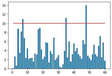
alpha tuning for weighted MSE

alpha_list = []
smape_list = []
for i in tqdm(range(60)):
    y = train.loc[train.num == i+1, 'power']
    x = train.loc[train.num == i+1, ].iloc[:, 3:]
    y_train, y_test, x_train, x_test = temporal_train_test_split(y = y, X = x, test_size = 168)
    xgb = XGBRegressor(seed = 0,
                      n_estimators = best_it[i], eta = 0.01, min_child_weight = xgb_params.iloc[i, 2],
                      max_depth = xgb_params.iloc[i, 3], colsample_bytree = xgb_params.iloc[i, 4], subsample = xgb_params.iloc[i, 5])
    
    xgb.fit(x_train, y_train)
    pred0 = xgb.predict(x_test)
    best_alpha = 0
    score0 = SMAPE(y_test,pred0)
    
    for j in [1, 3, 5, 7, 10, 25, 50, 75, 100]:
        xgb = XGBRegressor(seed = 0,
                      n_estimators = best_it[i], eta = 0.01, min_child_weight = xgb_params.iloc[i, 2],
                      max_depth = xgb_params.iloc[i, 3], colsample_bytree = xgb_params.iloc[i, 4], subsample = xgb_params.iloc[i, 5])
        xgb.set_params(**{'objective' : weighted_mse(j)})
    
        xgb.fit(x_train, y_train)
        pred1 = xgb.predict(x_test)
        score1 = SMAPE(y_test, pred1)
        if score1 < score0:
            best_alpha = j
            score0 = score1
    
    alpha_list.append(best_alpha)
    smape_list.append(score0)
    print("building {} || best score : {} || alpha : {}".format(i+1, score0, best_alpha))
  2%|█▍                                                                                 | 1/60 [00:13<13:19, 13.54s/it]
building 1 || best score : 0.14081881758107248 || alpha : 100
  3%|██▊                                                                                | 2/60 [00:19<08:54,  9.22s/it]
building 2 || best score : 2.6821957794380435 || alpha : 100
  5%|████▏                                                                              | 3/60 [00:29<09:06,  9.59s/it]
building 3 || best score : 0.6688717767933225 || alpha : 1
  7%|█████▌                                                                             | 4/60 [00:36<07:43,  8.28s/it]
building 4 || best score : 8.792995200216037 || alpha : 0
  8%|██████▉                                                                            | 5/60 [00:42<07:03,  7.70s/it]
building 5 || best score : 3.532240356378988 || alpha : 25
 10%|████████▎                                                                          | 6/60 [00:51<07:12,  8.00s/it]
building 6 || best score : 8.145093406219669 || alpha : 100
 12%|█████████▋                                                                         | 7/60 [01:03<08:21,  9.47s/it]
building 7 || best score : 10.928395316019108 || alpha : 75
 13%|███████████                                                                        | 8/60 [01:09<07:17,  8.42s/it]
building 8 || best score : 6.746168443992821 || alpha : 100
 15%|████████████▍                                                                      | 9/60 [01:23<08:38, 10.17s/it]
building 9 || best score : 2.3215949007391536 || alpha : 25
 17%|█████████████▋                                                                    | 10/60 [01:30<07:24,  8.89s/it]
building 10 || best score : 4.462851539347372 || alpha : 75
 18%|███████████████                                                                   | 11/60 [01:33<05:54,  7.23s/it]
building 11 || best score : 2.1730275177653446 || alpha : 3
 20%|████████████████▍                                                                 | 12/60 [01:39<05:30,  6.89s/it]
building 12 || best score : 2.258418884886762 || alpha : 3
 22%|█████████████████▊                                                                | 13/60 [01:45<05:14,  6.70s/it]
building 13 || best score : 2.3616037305351485 || alpha : 100
 23%|███████████████████▏                                                              | 14/60 [01:52<05:02,  6.59s/it]
building 14 || best score : 1.5336129579346058 || alpha : 0
 25%|████████████████████▌                                                             | 15/60 [01:55<04:14,  5.67s/it]
building 15 || best score : 3.296541983452375 || alpha : 7
 27%|█████████████████████▊                                                            | 16/60 [02:11<06:18,  8.60s/it]
building 16 || best score : 3.0680545392303955 || alpha : 3
 28%|███████████████████████▏                                                          | 17/60 [02:20<06:18,  8.80s/it]
building 17 || best score : 8.740441799973512 || alpha : 100
 30%|████████████████████████▌                                                         | 18/60 [02:30<06:24,  9.16s/it]
building 18 || best score : 8.94679591276322 || alpha : 0
 32%|█████████████████████████▉                                                        | 19/60 [02:40<06:22,  9.34s/it]
building 19 || best score : 4.226583737337153 || alpha : 0
 33%|███████████████████████████▎                                                      | 20/60 [02:47<05:49,  8.73s/it]
building 20 || best score : 2.0873767355223594 || alpha : 100
 35%|████████████████████████████▋                                                     | 21/60 [03:03<07:01, 10.80s/it]
building 21 || best score : 2.6544099712538256 || alpha : 0
 37%|██████████████████████████████                                                    | 22/60 [03:11<06:27, 10.20s/it]
building 22 || best score : 5.797805232965712 || alpha : 100
 38%|███████████████████████████████▍                                                  | 23/60 [03:29<07:34, 12.28s/it]
building 23 || best score : 5.6569368719345485 || alpha : 3
 40%|████████████████████████████████▊                                                 | 24/60 [03:42<07:35, 12.65s/it]
building 24 || best score : 1.360441026846758 || alpha : 100
 42%|██████████████████████████████████▏                                               | 25/60 [03:49<06:18, 10.82s/it]
building 25 || best score : 3.840535832896383 || alpha : 100
 43%|███████████████████████████████████▌                                              | 26/60 [03:56<05:28,  9.67s/it]
building 26 || best score : 3.213553180355984 || alpha : 75
 45%|████████████████████████████████████▉                                             | 27/60 [04:00<04:29,  8.16s/it]
building 27 || best score : 6.830400291873698 || alpha : 100
 47%|██████████████████████████████████████▎                                           | 28/60 [04:05<03:46,  7.07s/it]
building 28 || best score : 1.874738226904215 || alpha : 75
 48%|███████████████████████████████████████▋                                          | 29/60 [04:08<03:07,  6.05s/it]
building 29 || best score : 2.3391853032965058 || alpha : 3
 50%|█████████████████████████████████████████                                         | 30/60 [04:13<02:44,  5.49s/it]
building 30 || best score : 2.9692601738954028 || alpha : 10
 52%|██████████████████████████████████████████▎                                       | 31/60 [04:25<03:41,  7.64s/it]
building 31 || best score : 0.4073380176766228 || alpha : 100
 53%|███████████████████████████████████████████▋                                      | 32/60 [04:35<03:48,  8.16s/it]
building 32 || best score : 0.1971236790425161 || alpha : 50
 55%|█████████████████████████████████████████████                                     | 33/60 [04:52<04:52, 10.82s/it]
building 33 || best score : 0.9105866224713446 || alpha : 5
 57%|██████████████████████████████████████████████▍                                   | 34/60 [04:55<03:40,  8.48s/it]
building 34 || best score : 3.9267768501101448 || alpha : 25
 58%|███████████████████████████████████████████████▊                                  | 35/60 [05:05<03:42,  8.91s/it]
building 35 || best score : 11.234351213134072 || alpha : 100
 60%|█████████████████████████████████████████████████▏                                | 36/60 [05:13<03:31,  8.83s/it]
building 36 || best score : 2.458946897674616 || alpha : 75
 62%|██████████████████████████████████████████████████▌                               | 37/60 [05:26<03:47,  9.91s/it]
building 37 || best score : 5.9890804053673845 || alpha : 50
 63%|███████████████████████████████████████████████████▉                              | 38/60 [05:35<03:31,  9.61s/it]
building 38 || best score : 1.5342876060436252 || alpha : 100
 65%|█████████████████████████████████████████████████████▎                            | 39/60 [06:05<05:31, 15.78s/it]
building 39 || best score : 3.158475758619713 || alpha : 10
 67%|██████████████████████████████████████████████████████▋                           | 40/60 [06:11<04:20, 13.04s/it]
building 40 || best score : 5.500989373164019 || alpha : 1
 68%|████████████████████████████████████████████████████████                          | 41/60 [06:17<03:25, 10.80s/it]
building 41 || best score : 3.819655493226548 || alpha : 10
 70%|█████████████████████████████████████████████████████████▍                        | 42/60 [06:21<02:38,  8.83s/it]
building 42 || best score : 4.495863544380833 || alpha : 10
 72%|██████████████████████████████████████████████████████████▊                       | 43/60 [06:27<02:14,  7.90s/it]
building 43 || best score : 3.1305890374440746 || alpha : 75
 73%|████████████████████████████████████████████████████████████▏                     | 44/60 [06:41<02:35,  9.70s/it]
building 44 || best score : 2.718625179590631 || alpha : 0
 75%|█████████████████████████████████████████████████████████████▌                    | 45/60 [06:49<02:16,  9.11s/it]
building 45 || best score : 2.145678037348569 || alpha : 7
 77%|██████████████████████████████████████████████████████████████▊                   | 46/60 [07:01<02:22, 10.18s/it]
building 46 || best score : 6.3074642155568155 || alpha : 0
 78%|████████████████████████████████████████████████████████████████▏                 | 47/60 [07:13<02:16, 10.52s/it]
building 47 || best score : 5.399976988768882 || alpha : 100
 80%|█████████████████████████████████████████████████████████████████▌                | 48/60 [07:20<01:55,  9.66s/it]
building 48 || best score : 14.001549170839803 || alpha : 100
 82%|██████████████████████████████████████████████████████████████████▉               | 49/60 [07:29<01:42,  9.32s/it]
building 49 || best score : 2.8158476602820204 || alpha : 100
 83%|████████████████████████████████████████████████████████████████████▎             | 50/60 [07:37<01:29,  8.98s/it]
building 50 || best score : 2.333352911499234 || alpha : 25
 85%|█████████████████████████████████████████████████████████████████████▋            | 51/60 [07:49<01:28,  9.84s/it]
building 51 || best score : 1.8847318508795181 || alpha : 100
 87%|███████████████████████████████████████████████████████████████████████           | 52/60 [07:57<01:13,  9.23s/it]
building 52 || best score : 3.166745238923531 || alpha : 100
 88%|████████████████████████████████████████████████████████████████████████▍         | 53/60 [08:06<01:04,  9.21s/it]
building 53 || best score : 5.267101720487982 || alpha : 100
 90%|█████████████████████████████████████████████████████████████████████████▊        | 54/60 [08:15<00:54,  9.16s/it]
building 54 || best score : 3.1900609978512198 || alpha : 100
 92%|███████████████████████████████████████████████████████████████████████████▏      | 55/60 [08:22<00:42,  8.54s/it]
building 55 || best score : 2.709697897924913 || alpha : 100
 93%|████████████████████████████████████████████████████████████████████████████▌     | 56/60 [08:29<00:32,  8.01s/it]
building 56 || best score : 4.9618330667668245 || alpha : 100
 95%|█████████████████████████████████████████████████████████████████████████████▉    | 57/60 [08:40<00:26,  8.97s/it]
building 57 || best score : 7.171788489219123 || alpha : 100
 97%|███████████████████████████████████████████████████████████████████████████████▎  | 58/60 [08:45<00:15,  7.90s/it]
building 58 || best score : 2.492641662302252 || alpha : 100
 98%|████████████████████████████████████████████████████████████████████████████████▋ | 59/60 [08:48<00:06,  6.46s/it]
building 59 || best score : 5.739513120433657 || alpha : 3
100%|██████████████████████████████████████████████████████████████████████████████████| 60/60 [08:55<00:00,  8.92s/it]
building 60 || best score : 1.7586635594500057 || alpha : 3

no_df = pd.DataFrame({'score':smape_list})
plt.bar(np.arange(len(no_df))+1, no_df['score'])
plt.plot([1,60], [10, 10], color = 'red')
[<matplotlib.lines.Line2D at 0x27a739b7550>]

4. test inference

preprocessing for test data

# train set과 동일한 전처리 과정
test = pd.read_csv('./data/test.csv', encoding = 'cp949')
cols = ['num', 'date_time', 'temp', 'wind','hum' ,'prec', 'sun', 'non_elec', 'solar']
test.columns = cols
date = pd.to_datetime(test.date_time)
test['hour'] = date.dt.hour
test['day'] = date.dt.weekday
test['month'] = date.dt.month
test['week'] = date.dt.weekofyear
test['sin_time'] = np.sin(2*np.pi*test.hour/24)
test['cos_time'] = np.cos(2*np.pi*test.hour/24)
test['holiday'] = test.apply(lambda x : 0 if x['day']<5 else 1, axis = 1)
test.loc[('2020-08-17'<=test.date_time)&(test.date_time<'2020-08-18'), 'holiday'] = 1

## 건물별 일별 시간별 발전량 평균
tqdm.pandas()
test['day_hour_mean'] = test.progress_apply(lambda x : power_mean.loc[(power_mean.num == x['num']) & (power_mean.day == x['day']) & (power_mean.hour == x['hour']) ,'power'].values[0], axis = 1)

## 건물별 시간별 발전량 평균 넣어주기
tqdm.pandas()
test['hour_mean'] = test.progress_apply(lambda x : power_hour_mean.loc[(power_hour_mean.num == x['num']) & (power_hour_mean.hour == x['hour']) ,'power'].values[0], axis = 1)

tqdm.pandas()
test['hour_std'] = test.progress_apply(lambda x : power_hour_std.loc[(power_hour_std.num == x['num']) & (power_hour_std.hour == x['hour']) ,'power'].values[0], axis = 1)

test.drop(['non_elec', 'solar','hour','date_time'], axis = 1, inplace = True)

# pandas 내 선형보간 method 사용
for i in range(60):
    test.iloc[i*168:(i+1)*168, :]  = test.iloc[i*168:(i+1)*168, :].interpolate()


test['THI'] = 9/5*test['temp'] - 0.55*(1-test['hum']/100)*(9/5*test['hum']-26)+32

cdhs = np.array([])
for num in range(1,61,1):
    temp = test[test['num'] == num]
    cdh = CDH(temp['temp'].values)
    cdhs = np.concatenate([cdhs, cdh])
test['CDH'] = cdhs

test = test[['num','temp', 'wind', 'hum', 'prec', 'sun', 'day', 'month', 'week',
       'day_hour_mean', 'hour_mean', 'hour_std', 'holiday', 'sin_time',
       'cos_time', 'THI', 'CDH']]
test.head()
<ipython-input-18-16a57dad2551>:9: FutureWarning: Series.dt.weekofyear and Series.dt.week have been deprecated.  Please use Series.dt.isocalendar().week instead.
  test['week'] = date.dt.weekofyear
100%|██████████████████████████████████████████████████████████████████████████| 10080/10080 [00:05<00:00, 1800.18it/s]
100%|██████████████████████████████████████████████████████████████████████████| 10080/10080 [00:03<00:00, 2751.89it/s]
100%|██████████████████████████████████████████████████████████████████████████| 10080/10080 [00:03<00:00, 2778.56it/s]
num temp wind hum prec sun day month week day_hour_mean hour_mean hour_std holiday sin_time cos_time THI CDH
0 1 27.800000 1.500000 74.000000 0.0 0.0 1 8 35 8505.972 8540.373176 118.793252 0 0.000000 1.000000 66.710400 1.800000
1 1 27.633333 1.366667 75.333333 0.0 0.0 1 8 35 8442.414 8517.174776 137.989738 0 0.258819 0.965926 66.870933 3.433333
2 1 27.466667 1.233333 76.666667 0.0 0.0 1 8 35 8475.948 8509.055718 122.381197 0 0.500000 0.866025 67.066667 4.900000
3 1 27.300000 1.100000 78.000000 0.0 0.0 1 8 35 8444.844 8493.313129 122.054777 0 0.707107 0.707107 67.297600 6.200000
4 1 26.900000 1.166667 79.666667 0.0 0.0 1 8 35 8425.242 8479.522165 124.472447 0 0.866025 0.500000 67.290767 7.100000
xgb_params['alpha'] = alpha_list
xgb_params['best_it'] = best_it
xgb_params.head()
n_estimators eta min_child_weight max_depth colsample_bytree subsample alpha best_it
0 100 0.01 4 5 0.8 0.8 100 1051
1 100 0.01 6 3 0.8 0.9 100 534
2 100 0.01 6 7 0.9 0.9 1 637
3 100 0.01 3 7 0.8 0.9 0 379
4 100 0.01 2 6 0.9 0.9 25 447
#xgb_params.to_csv('./hyperparameter_xgb_final.csv', index=False)
## best hyperparameters 불러오기
xgb_params = pd.read_csv('./parameters/hyperparameter_xgb_final.csv')
xgb_params.head()
n_estimators eta min_child_weight max_depth colsample_bytree subsample alpha best_it
0 100 0.01 4 5 0.8 0.8 100 1051
1 100 0.01 6 3 0.8 0.9 100 534
2 100 0.01 6 7 0.9 0.9 1 637
3 100 0.01 3 7 0.8 0.9 0 379
4 100 0.01 2 6 0.9 0.9 25 447
best_it = xgb_params['best_it'].to_list()
best_it[0]        # 1051
1051

seed ensemble

- seed별로 예측값이 조금씩 바뀝니다.

- seed의 영향을 제거하기 위해 6개의 seed(0부터 5)별로 훈련, 예측하여 6개 예측값의 평균을 구했습니다.

preds = np.array([]) 
for i in tqdm(range(60)):
    
    pred_df = pd.DataFrame()   # 시드별 예측값을 담을 data frame
    
    for seed in [0,1,2,3,4,5]: # 각 시드별 예측
        y_train = train.loc[train.num == i+1, 'power']
        x_train, x_test = train.loc[train.num == i+1, ].iloc[:, 3:], test.loc[test.num == i+1, ].iloc[:,1:]
        x_test = x_test[x_train.columns]
        
        xgb = XGBRegressor(seed = seed, n_estimators = best_it[i], eta = 0.01, 
                           min_child_weight = xgb_params.iloc[i, 2], max_depth = xgb_params.iloc[i, 3], 
                           colsample_bytree=xgb_params.iloc[i, 4], subsample=xgb_params.iloc[i, 5])
    
        if xgb_params.iloc[i,6] != 0:  # 만약 alpha가 0이 아니면 weighted_mse 사용
            xgb.set_params(**{'objective':weighted_mse(xgb_params.iloc[i,6])})
        
        xgb.fit(x_train, y_train)
        y_pred = xgb.predict(x_test)
        pred_df.loc[:,seed] = y_pred   # 각 시드별 예측 담기
        
    pred = pred_df.mean(axis=1)        # (i+1)번째 건물의 예측 =  (i+1)번째 건물의 각 시드별 예측 평균값
    preds = np.append(preds, pred)   
100%|██████████████████████████████████████████████████████████████████████████████████| 60/60 [05:42<00:00,  5.70s/it]
preds = pd.Series(preds)

fig, ax = plt.subplots(60, 1, figsize=(100,200), sharex = True)
ax = ax.flatten()
for i in range(60):
    train_y = train.loc[train.num == i+1, 'power'].reset_index(drop = True)
    test_y = preds[i*168:(i+1)*168]
    ax[i].scatter(np.arange(2040) , train.loc[train.num == i+1, 'power'])
    ax[i].scatter(np.arange(2040, 2040+168) , test_y)
    ax[i].tick_params(axis='both', which='major', labelsize=6)
    ax[i].tick_params(axis='both', which='minor', labelsize=4)
#plt.savefig('./predict_xgb.png')
plt.show()
submission = pd.read_csv('./data/sample_submission.csv')
submission['answer'] = preds
submission.to_csv('./submission/submission_xgb_noclip.csv', index = False)

5. post processing

weighted mse와 같은 맥락에서, 과도한 underestimate를 막기 위해 예측값을 후처리했습니다.

- 예측 주로부터 직전 4주(train set 마지막 28일)의 건물별 요일별 시간대별 전력소비량의 최솟값을 구한 뒤,
- test set의 같은 건물 요일 시간대의 예측값과 비교하여 만약 1번의 최솟값보다 예측값이 작다면 최솟값으로 예측값을 대체해주었습니다.
- public score 0.01 , private score 0.08 정도의 성능 향상이 있었습니다.
train_to_post = pd.read_csv('./data/train.csv', encoding = 'cp949')
cols = ['num', 'date_time', 'power', 'temp', 'wind','hum' ,'prec', 'sun', 'non_elec', 'solar']
train_to_post.columns = cols
date = pd.to_datetime(train_to_post.date_time)
train_to_post['hour'] = date.dt.hour
train_to_post['day'] = date.dt.weekday
train_to_post['month'] = date.dt.month
train_to_post['week'] = date.dt.weekofyear
train_to_post = train_to_post.loc[(('2020-08-17'>train_to_post.date_time)|(train_to_post.date_time>='2020-08-18')), ].reset_index(drop = True)

pred_clip = []
test_to_post = pd.read_csv('./data/test.csv',  encoding = 'cp949')
cols = ['num', 'date_time', 'temp', 'wind','hum' ,'prec', 'sun', 'non_elec', 'solar']
test_to_post.columns = cols
date = pd.to_datetime(test_to_post.date_time)
test_to_post['hour'] = date.dt.hour
test_to_post['day'] = date.dt.weekday
test_to_post['month'] = date.dt.month
test_to_post['week'] = date.dt.weekofyear

## submission 불러오기
df = pd.read_csv('./submission/submission_xgb_noclip.csv')
for i in range(60):
    min_data = train_to_post.loc[train_to_post.num == i+1, ].iloc[-28*24:, :] ## 건물별로 직전 28일의 데이터 불러오기
    ## 요일별, 시간대별 최솟값 계산
    min_data = pd.pivot_table(min_data, values = 'power', index = ['day', 'hour'], aggfunc = min).reset_index() 
    pred = df.answer[168*i:168*(i+1)].reset_index(drop=True) ## 168개 데이터, 즉 건물별 예측값 불러오기
    day =  test_to_post.day[168*i:168*(i+1)].reset_index(drop=True) ## 예측값 요일 불러오기
    hour = test_to_post.hour[168*i:168*(i+1)].reset_index(drop=True) ## 예측값 시간 불러오기
    df_pred = pd.concat([pred, day, hour], axis = 1)
    df_pred.columns = ['pred', 'day', 'hour']
    for j in range(len(df_pred)):
        min_power = min_data.loc[(min_data.day == df_pred.day[j])&(min_data.hour == df_pred.hour[j]), 'power'].values[0]
        if df_pred.pred[j] < min_power:
            pred_clip.append(min_power)
        else:
            pred_clip.append(df_pred.pred[j])
<ipython-input-26-2e13e7f53e14>:8: FutureWarning: Series.dt.weekofyear and Series.dt.week have been deprecated.  Please use Series.dt.isocalendar().week instead.
  train_to_post['week'] = date.dt.weekofyear
<ipython-input-26-2e13e7f53e14>:19: FutureWarning: Series.dt.weekofyear and Series.dt.week have been deprecated.  Please use Series.dt.isocalendar().week instead.
  test_to_post['week'] = date.dt.weekofyear
초록색으로 표시된 값이 원래의 예측값, 주황색이 후처리된 예측값입니다.
변동이 거의 없는 건물도 있으나, 유의미하게 바뀐 건물도 확인됩니다.
pred_origin = df.answer
pred_clip = pd.Series(pred_clip)
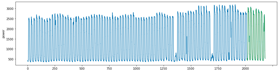
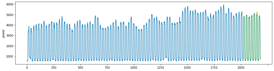
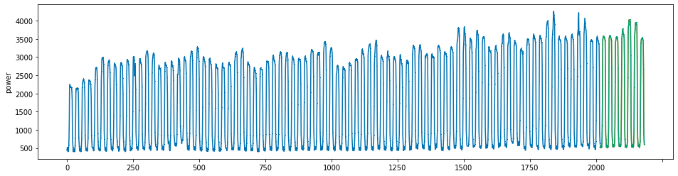
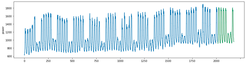
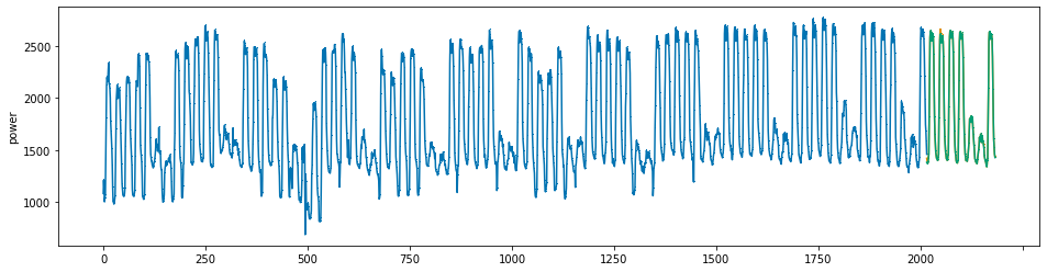
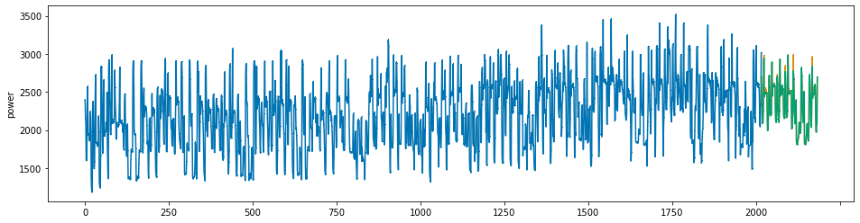
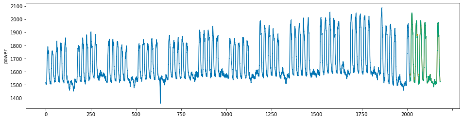
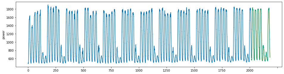
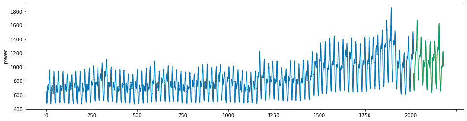
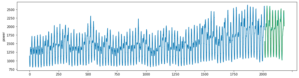
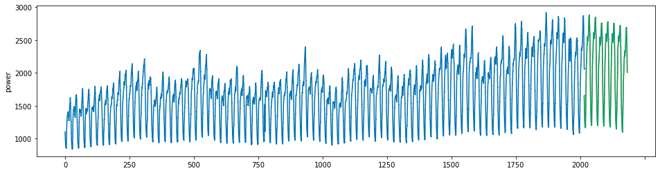
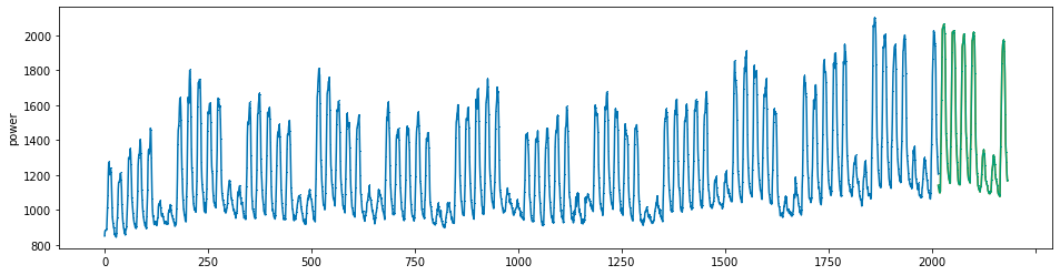
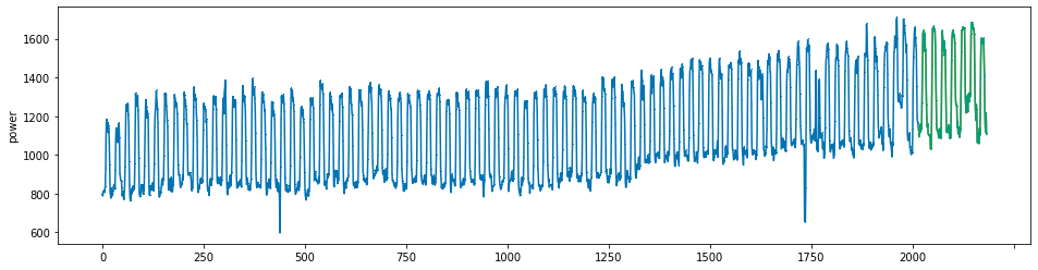
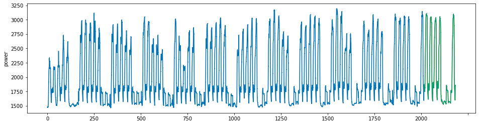
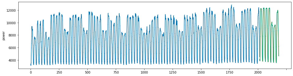
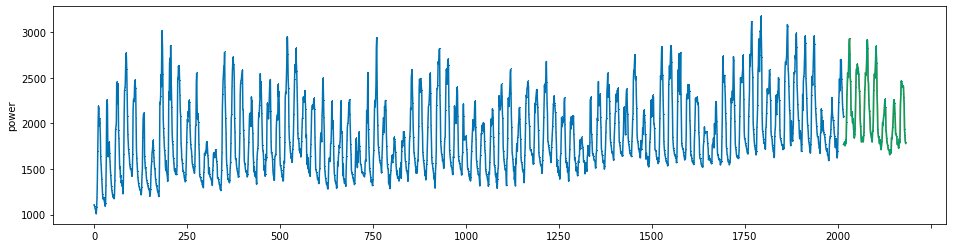
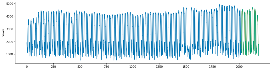
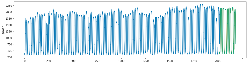
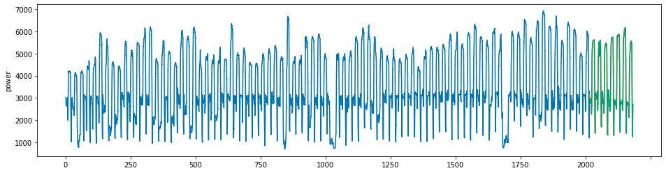
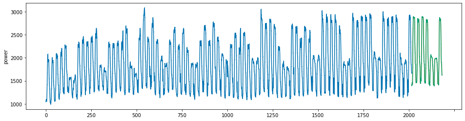
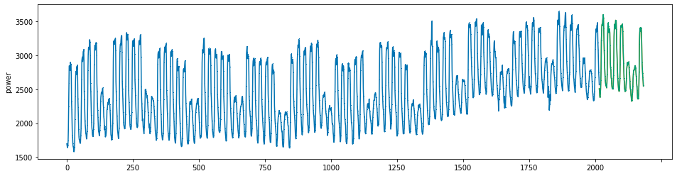
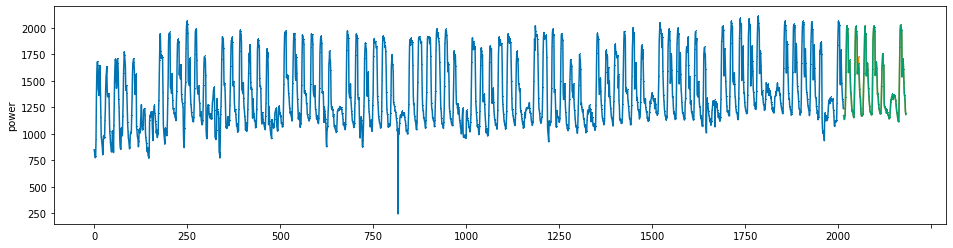
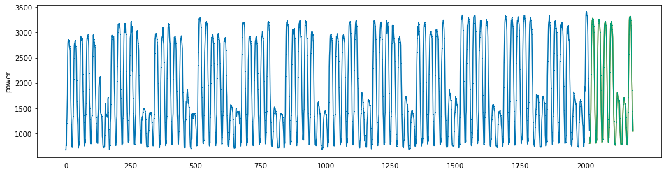
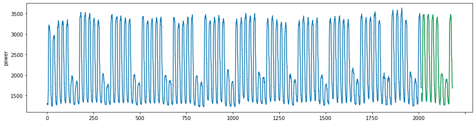
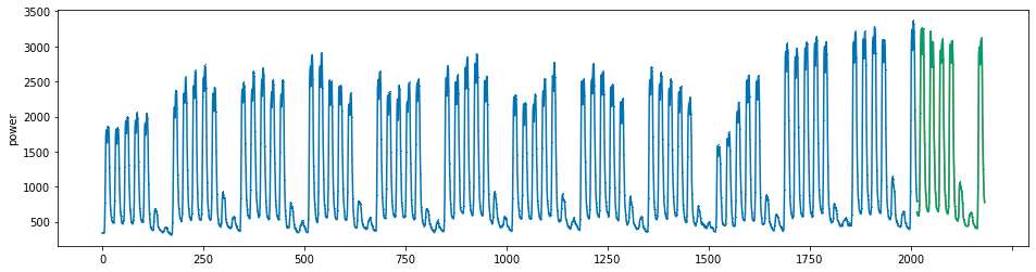
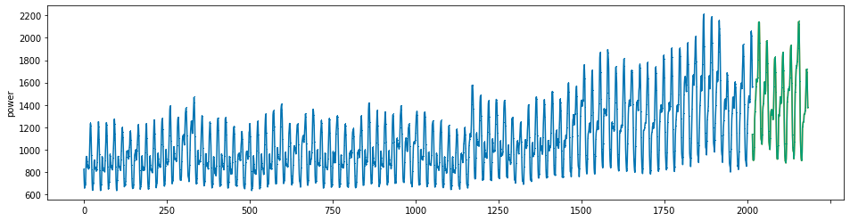
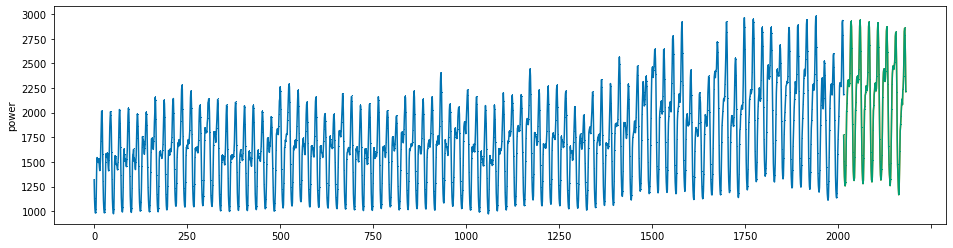
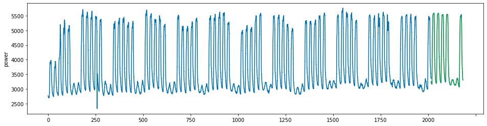
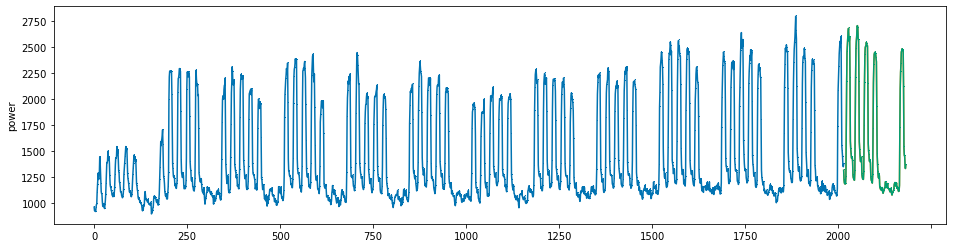
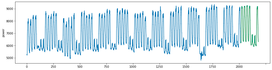
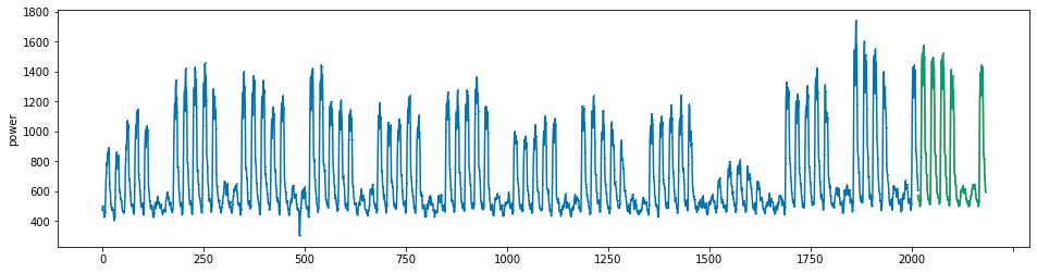
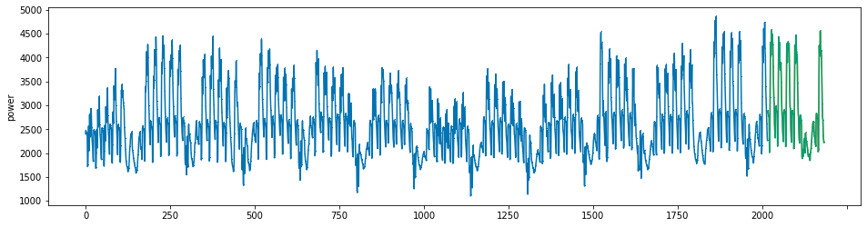
for i in range(60):
    power = train_to_post.loc[train_to_post.num == i+1, 'power'].reset_index(drop=True)
    preds = pred_clip[i*168:(i+1)*168]
    preds_origin = pred_origin[i*168:(i+1)*168]
    preds.index = range(power.index[-1], power.index[-1]+168)
    preds_origin.index = range(power.index[-1], power.index[-1]+168)
    
    plot_series(power, preds,  preds_origin, markers = [',', ',', ','])
C:\Users\HS\anaconda3\envs\reproduce\lib\site-packages\sktime\utils\plotting.py:80: RuntimeWarning: More than 20 figures have been opened. Figures created through the pyplot interface (`matplotlib.pyplot.figure`) are retained until explicitly closed and may consume too much memory. (To control this warning, see the rcParam `figure.max_open_warning`).
  fig, ax = plt.subplots(1, figsize=plt.figaspect(0.25))

create submission file

submission = pd.read_csv('./data/sample_submission.csv')
submission['answer'] = pred_clip
submission.to_csv('./submission//submission_xgb_final.csv', index = False)