데이터 : 전력거래소 시간대별 수요량 데이터 활용 기간 : 2013-2021년
In [29]:
import numpy as np
import pandas as pd
from datetime import datetime, date
import datetime

import matplotlib.pyplot as plt
import seaborn as sns
In [30]:
plt.rcParams['figure.figsize'] = (14, 9)
plt.rcParams['font.family'] = 'Malgun Gothic'
plt.rcParams['font.size'] = 12
plt.rcParams['axes.unicode_minus']
Out[30]:
In [31]:
df = pd.read_excel('시간별 전력수요량_2013_2021.xlsx', index_col=[0], parse_dates=True)
df
Out[31]:
In [32]:
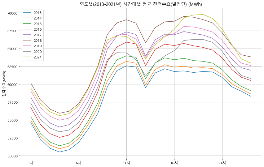
# (전체) 2013-2021년 시간대별 부하곡선, 부하율
def series_year_profit(data, type): # (0 비정규화(소비량), 1 정규화(부하률)
for idx in data.index.year.unique(): # 2013년부터 2021년까지 순차 반복
df_pf = data[str(idx)]
if type == 0:
df_pf.mean().plot(label=idx)
plt.ylabel('전력수요(MWh)')
plt.title('연도별(2013-2021년) 시간대별 평균 전력수요(발전단) (MWh)')
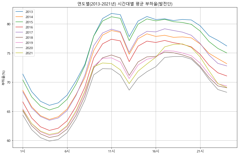
if type == 1:
df_pf = df_pf / df_pf.max(axis=0).max() *100 # 연 최대값으로 나누어 정규화
df_pf.mean().plot(label=idx)
plt.ylabel('부하율(%)')
plt.title('연도별(2013-2021년) 시간대별 평균 부하율(발전단)')
plt.legend()
plt.grid()
plt.show()
In [33]:
series_year_profit(df.copy(), 0) # 비정규화(소비량)
In [34]:
series_year_profit(df.copy(), 1) # 정규화(부하율)
In [35]:
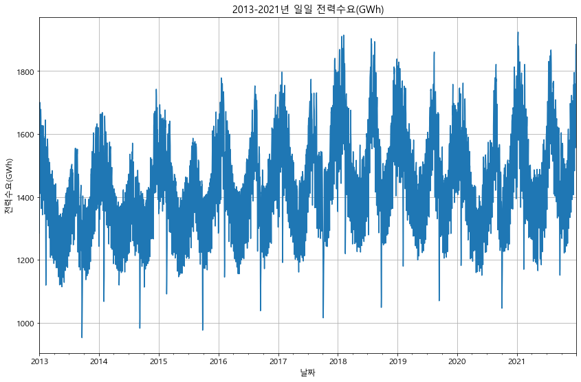
# (전체) 2013-2021년 일별 전력소비량 라인 그래프
def multi_year_daily_consumption(multi):
    multi['sum'] = multi.sum(axis=1) / 1000 # MWh를 GWh로 변경
    multi['sum'].plot() # 일일 전력소비량 그리기
    plt.grid()
    plt.ylabel('전력수요(GWh)')
    plt.title('2013-2021년 일일 전력수요(GWh)')
    plt.show()
In [36]:
multi_year_daily_consumption(df.copy())
In [37]:
# (전체) 2013-2021년 월별 막대그래프
def multi_year_month_consumption(multi):
    multi['sum'] = multi.sum(axis=1) / 1000 # MWh를 GWh로 변경

    multi['year'] = multi.index.year # 연도 컬럼 생성
    multi['month'] = multi.index.month # 월 컬럼 생성
    #print(multi)
    grp_multi = multi.groupby(['year', 'month'])['sum'].sum() # 연도, 월별 합계 계산
    grp_multi = pd.DataFrame(grp_multi)
    grp_multi = grp_multi.reset_index()

    sns.barplot(data=grp_multi, x='month', y='sum', hue='year') # 멀티 막대 그래프 그리기

    plt.grid()
    plt.ylabel('전력수요(GWh)')
    plt.title('2013-2021년 월별 전력수요(GWh)')
    plt.show()
In [38]:
multi_year_month_consumption(df.copy())

In [39]:
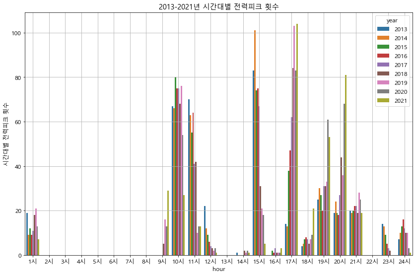
# (전체) 시간대별 전력피크 횟수 계산
def count_peak_month(data):
    data['year'] = data.index.year
    data['peak'] = data.idxmax(axis=1)  # 하루 중 최고값을 기록한 시간을 추출

    total = pd.DataFrame(index=data.columns)

    for idx in data['year'].unique():
        year = data[data['year'] == idx]  # 연도별 데이터

        peak_hour = year['peak'].value_counts()  # 'peak' 컬럼에 있는 값별 count
        peak_hour = pd.DataFrame(peak_hour)

        total = pd.concat([total, peak_hour], axis=1)  # 연도별로 계속 결합

    total.columns = data['year'].unique()  # 전체 연도를 컬럼으로 변경
    total = total.fillna(0)  # 피크가 기록되지 않은 시간대의 Nan 값을 0으로 변경
    total = total.T.drop(['year', 'peak'], axis=1)  # 행/열 전환
    total = total.stack().reset_index()  # 열('시간')을 행으로 전환하고, idnex를 reset
    total.columns = ['year', 'hour', 'count']  # 컬럼명 변경

    sns.barplot(data=total, x='hour', y='count', hue='year')  # 멀티 막대 그래프 그리기

    plt.grid()
    plt.ylabel('시간대별 전력피크 횟수')
    plt.title('2013-2021년 시간대별 전력피크 횟수')
    plt.show()
In [40]:
count_peak_month(df.copy())
In [48]:
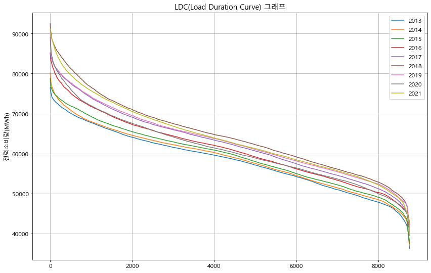
# (전체) LDC(Load Duration Curve) 그래프
def ldc(df_ldc):
    df_ldc = df_ldc.stack()
    df_ldc = df_ldc.reset_index()
    df_ldc.columns = ['date', 'hour', 'pcon']
    df_ldc['year'] = df_ldc.date.dt.year

    ldc = pd.DataFrame()
    for idx in df_ldc['year'].unique():
        temp = df_ldc[df_ldc['year'] == idx] # 해당년도 데이터
        ldc[idx] = temp['pcon'].sort_values(ascending=False).reset_index(drop=True)
        # 전력소비량을 sort_values로 정렬, reset_index(drop=True)로 index 삭제해 0, 1, 3 순서 설정

    ldc.plot()
    plt.grid()
    plt.legend()
    plt.ylabel('전력소비량(MWh)')
    plt.title('LDC(Load Duration Curve) 그래프')
    plt.show()
In [49]:
ldc(df.copy())